LowLevelFEM

LowLevelFEM is a Julia package for finite element analysis with an engineering-first workflow, designed to assemble finite element operators explicitly at matrix and field level. It exposes each phase of the workflow as simple functions (mesh → matrices → loads/BCs → solve → postprocess → visualize), so you can customize, combine, or inspect any step at matrix and field level. Typical tasks such as strain energy or resultants are one-liners (for example, U = q' * K * q / 2). The package is suitable not only for classical structural mechanics problems, but also for rapid assembly of general linear PDEs expressed in weak form.

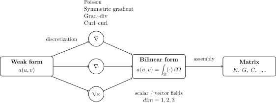
Operator-level finite element workflow in LowLevelFEM. Weak forms are discretized into elementary differential operators (grad, div, curl), which are assembled into bilinear forms and global system matrices.

Documentation Map

• Getting Started
• Tutorials
• Manual
• API Reference
• Explanations
• News

Requirements

• Julia 1.x
• Gmsh C API is bundled via gmsh_jll and re-exported as gmsh from this package; no separate Gmsh.jl installation is required.

Citation

If you use LowLevelFEM.jl in academic work, please cite the accompanying JOSS paper:

Balázs Pere (2026). LowLevelFEM.jl: A lightweight finite element toolbox in Julia, Journal of Open Source Software, 11(123), 10096, https://doi.org/10.21105/joss.10096

A BibTeX entry is provided in CITATION.cff.

Capabilities

• Geometry and meshing: integrates with gmsh for 2D/3D geometry, meshing, and physical groups.
• Problem types: 3D solids, 2D plane stress/plane strain, axisymmetric; 3D/2D heat conduction and axisymmetric heat conduction.
• Elements and order: standard line/triangle/quad/tetra/hex/pyramid/wedge with Lagrange order up to 10.
• Materials: linear elastic (Hooke) and hyperelastic materials given by their free energy function. Direct input of 6×6 constitutive matrix is also possible.
• Matrices: stiffness K, mass M (lumped or consistent), proportional damping C (Rayleigh/Caughey), heat conduction/capacity, latent heat, convection matrices/vectors, and generic Poisson-type operators for scalar and vector fields.
• Explicit matrices and fields: unlike many high-level FEM packages, LowLevelFEM keeps global matrices and finite element fields accessible throughout the workflow, making every stage of the analysis transparent and customizable.
• Operator-level programming: implement, inspect and modify PDE operators, constitutive laws and weak-form formulations directly at matrix and field level.
• Loads and constraints: nodal and distributed loads on physical groups; function-based loads and temperature BCs; elastic supports; initial displacement/velocity/temperature.
• Thermal–structural coupling: thermal expansion, thermal stresses, and heat generated by elastic deformation.
• Solvers: static (direct and iterative solvers with arbitrary preconditioners) and transient dynamics (central difference and HHT-α from the Newmark family).
• Eigenproblems: modal analysis (frequencies and mode shapes, optionally prestressed) and linear buckling (critical factors and modes).
• Field operators and results: gradient/divergence/curl; stress/strain and heat flux as element or nodal fields; smoothing at nodes with field jumps; user-defined scalar/vector/tensor FE fields.
• Visualization and plots: Gmsh-based views for displacements, stresses, strains, heat flux, with animation for dynamics; plot results along user-defined paths; show results on surfaces.
• Coordinate systems: rotate nodal DOFs with constant or function-defined local coordinate systems (incl. curvilinear).
• Truss structures (static, transient, modal analysis)
• Nonlinear solid mechanics (Total Lagrangian formulation) Energy-based hyperelasticity with consistent stress and tangent operators, including geometric stiffness and follower loads for large-deformation problems.
• Weak-form assembly supports shared-memory multithreading. Bilinear forms use memory-efficient direct CSC assembly by default, while the triplet-based IJV method remains available as an option.

Installation

using Pkg
Pkg.add("LowLevelFEM")

Quick Start

using LowLevelFEM

structured_rect_mesh() # uses Gmsh to create mesh

mat = Material("body", E=2e5, ν=0.3)
prob = Problem([mat], type=:PlaneStrain)  # :Solid, :PlaneStress, :AxiSymmetric, :HeatConduction, ...

bc    = displacementConstraint("left", ux=0, uy=0)
force = load("right", fy=-1)

u = solveDisplacement(prob, load=[force], support=[bc])
S = solveStress(u)

showDoFResults(u, visible=true)
showDoFResults(u, :ux)
showStressResults(S)
showStressResults(S, :sxy, name="Shear stress")

openPostProcessor()

Note: physical group names in your geometry (created in Gmsh) must match the strings used above (e.g., "body", "left", "right").

An alternative solution (instead of u = ..., S = ...)

K = stiffnessMatrix(prob)
f = loadVector(prob, [force])
u = solveDisplacement(K, f, support=[bc])

E = mat.E
ν = mat.ν

u = expandTo3D(u)

A = (u ∘ ∇ + ∇ ∘ u) / 2
I = TensorField(prob, "body", [1 0 0; 0 1 0; 0 0 1])
S = E / (1 + ν) * (A + ν / (1 - 2ν) * trace(A) * I)

Operator-level weak-form assembly

For custom PDEs and multifield formulations, the finite element operator can also be assembled directly from its weak form. Differential operators and coefficient matrices remain explicit, allowing the formulation to be inspected, modified and combined without implementing a dedicated solver.

Pu = Problem([mat], type=:VectorField, dim=2, field=:u)

E = mat.E
ν = mat.ν

C = E / ((1 + ν) * (1 - 2ν)) * [
    1-ν  ν    0
    ν    1-ν  0
    0    0    (1-2ν)/2
]

K = ∫(SymGrad(Pu) ⋅ C ⋅ SymGrad(Pu), Ω="body")
f = ∫(Pu ⋅ [0, -1], Γ="right")
bc = BoundaryCondition("left", ux=0, uy=0)

u = solveField(K, f, support=[bc])

Bilinear forms are assembled directly into CSC sparse matrices by default. This reduces temporary memory use and allows substantially larger problems than triplet-based assembly. For repeated assembly on the same mesh and field pair, the sparsity pattern can be built once and reused:

Kpattern = build_csc_pattern(Pu, Pu; Ω="body")

fill!(Kpattern.nzval, 0.0)
K = ∫(SymGrad(Pu) ⋅ C ⋅ SymGrad(Pu);
      Ω="body", csc_matrix=Kpattern)

The pattern must retain its structural zeros; do not call dropzeros! on it. Before an independent reuse, reset its numerical values with fill! as shown above. The previous triplet route remains available with assembly=:ijv.

The three examples above solve the same class of problem at different levels of abstraction:

1. predefined engineering solver,
2. explicit matrices and finite element fields,
3. direct weak-form operator assembly.

The higher-level functions are convenience wrappers; the underlying matrices, fields and operators remain accessible throughout the workflow.

For interactive work with custom geometries

Gmsh can be launched directly from Julia.

openGeometry("test.geo")
openPreProcessor()

If test.geo already exists, it is opened for editing. Otherwise, openGeometry automatically creates a new geometry file, which can then be edited in Gmsh using openPreProcessor().

This workflow is recommended for custom geometries and more advanced finite element models.

More end-to-end examples, tutorials and application notebooks are available in the examples directory and the online documentation.

Documentation

• Latest docs: https://perebalazs.github.io/LowLevelFEM.jl/dev
• Stable docs: https://perebalazs.github.io/LowLevelFEM.jl/stable

Planned features

• Hierarchical H1/H2 approximation for beam and shell formulations
• Contact problems (penalty, Lagrange multiplier)

Any suggestions are welcome. In case of any issue, please send a bug report.

License

This project is licensed under the MIT License — see LICENSE for details.